Overview of Python
Python is interpreted
Python is an interpreted language, in contrast to Java and C which are compiled languages.
This means we can type statements into the interpreter and they are executed immediately.
5 + 5
- Groups of statements are all executed one after the other:
x = 5
y = 'Hello There'
z = 10.5
- We can visualize the above code using PythonTutor.
x + 5
Assignments versus equations
In Python when we write
x = 5this means something different from an equation $x=5$.Unlike variables in mathematical models, variables in Python can refer to different things as more statements are interpreted.
x = 1
print('The value of x is', x)

x = 2.5
print('Now the value of x is', x)

x = 'hello there'
print('Now it is ', x)
Calling Functions
We can call functions in a conventional way using round brackets
round(3.14)
Types
Values in Python have an associated type.
If we combine types incorrectly we get an error.
print(y)
y + 5
The type function
- We can query the type of a value using the
typefunction.
type(1)
type('hello')
type(2.5)
type(True)
Null values
Sometimes we represent "no data" or "not applicable".
In Python we use the special value
None.This corresponds to
Nullin Java or SQL.
result = None
- When we fetch the value
Nonein the interactive interpreter, no result is printed out.
result
Testing for Null values
- We can check whether there is a result or not using the
isoperator:
result is None
x = 5
x is None
x = 1
x
type(x)
y = float(x)
y
Converting to integers
- To convert a floating-point to an integer use the
int()function.
type(y)
int(y)
Variables are not typed
- Variables themselves, on the other hand, do not have a fixed type.
- It is only the values that they refer to that have a type.
- This means that the type referred to by a variable can change as more statements are interpreted.
y = 'hello'
print('The type of the value referred to by y is ', type(y))
y = 5.0
print('And now the type of the value is ', type(y))
Polymorphism
- The meaning of an operator depends on the types we are applying it to.
1 + 1
'a' + 'b'
'1' + '1'
Conditional Statements and Indentation
The syntax for control structures in Python uses colons and indentation.
Beware that white-space affects the semantics of Python code.
Statements that are indented using the Tab key are grouped together.
if statements
x = 5
if x > 0:
    print('x is strictly positive.')
    print(x)

print('finished.')
- Visualize the above on PythonTutor.
Changing indentation
x = 0
if x > 0:
    print('x is strictly positive.')
print(x)

print('finished.')
- Visualize the above on PythonTutor.
if and else
x = 0
print('Starting.')
if x > 0:
    print('x is strictly positive.')
else:
    if x < 0:
        print('x is strictly negative.')
    else:
        print('x is zero.')
print('finished.')
- Visualize the above on PythonTutor.
elif
print('Starting.')
if x > 0:
    print('x is strictly positive')
elif x < 0:
    print('x is strictly negative')
else:
    print('x is zero')
print('finished.')
Lists
We can use lists to hold an ordered sequence of values.
l = ['first', 'second', 'third']
l
Lists can contain different types of variable, even in the same list.
another_list = ['first', 'second', 'third', 1, 2, 3]
another_list
Mutable Datastructures
Lists are mutable; their contents can change as more statements are interpreted.
l.append('fourth')
l
References
Whenever we bind a variable to a value in Python we create a reference.
A reference is distinct from the value that it refers to.
Variables are names for references.
X = [1, 2, 3]
Y = X
Side effects
The above code creates two different references (named
XandY) to the same value[1, 2, 3]Because lists are mutable, changing them can have side-effects on other variables.
If we append something to
Xwhat will happen toY?
X.append(4)
X
Y
- Visualize the above on PythonTutor.
State and identity
The state referred to by a variable is different from its identity.
To compare state use the
==operator.To compare identity use the
isoperator.When we compare identity we check equality of references.
When we compare state we check equality of values.
Example
- We will create two different lists, with two associated variables.
X = [1, 2]
Y = [1]
Y.append(2)
- Visualize the above code on PythonTutor.
Comparing state
X
Y
X == Y
Comparing identity
X is Y
Copying data prevents side effects
- In this example, because we have two different lists we avoid side effects
Y.append(3)
X
X == Y
X is Y
Iteration
- We can iterate over each element of a list in turn using a
forloop:
my_list = ['first', 'second', 'third', 'fourth']
for i in my_list:
    print(i)
- Visualize the above on PythonTutor.
Including more than one statement inside the loop
my_list = ['first', 'second', 'third', 'fourth']
for i in my_list:
    print("The next item is:")
    print(i)
    print()
- Visualize the above code on PythonTutor.
Looping a specified number of times
- To perform a statement a certain number of times, we can iterate over a list of the required size.
for i in [0, 1, 2, 3]:
    print("Hello!")
The range function
To save from having to manually write the numbers out, we can use the function
range()to count for us.We count starting at 0 (as in Java and C++).
list(range(4))
for loops with the range function
for i in range(4):
    print("Hello!")
List Indexing
- Lists can be indexed using square brackets to retrieve the element stored in a particular position.
my_list
my_list[0]
my_list[1]
List Slicing
We can also a specify a range of positions.
This is called slicing.
The example below indexes from position 0 (inclusive) to 2 (exclusive).
my_list[0:2]
Indexing from the start or end
- If we leave out the starting index it implies the beginning of the list:
my_list[:2]
- If we leave out the final index it implies the end of the list:
my_list[2:]
Copying a list
- We can conveniently copy a list by indexing from start to end:
new_list = my_list[:]
new_list
new_list is my_list
Negative Indexing
- Negative indices count from the end of the list:
my_list[-1]
my_list[:-1]
Collections
Lists are an example of a collection.
A collection is a type of value that can contain other values.
There are other collection types in Python:
tuplesetdict
Tuples
Tuples are another way to combine different values.
The combined values can be of different types.
Like lists, they have a well-defined ordering and can be indexed.
To create a tuple in Python, use round brackets instead of square brackets
tuple1 = (50, 'hello')
tuple1
tuple1[0]
type(tuple1)
Tuples are immutable
- Unlike lists, tuples are immutable. Once we have created a tuple we cannot add values to it.
tuple1.append(2)
Sets
Lists can contain duplicate values.
A set, in contrast, contains no duplicates.
Sets can be created from lists using the
set()function.
X = set([1, 2, 3, 3, 4])
X
type(X)
- Alternatively we can write a set literal using the
{and}brackets.
X = {1, 2, 3, 4}
type(X)
Sets are mutable
- Sets are mutable like lists:
X.add(5)
X
- Duplicates are automatically removed
X.add(5)
X
Sets are unordered
Sets do not have an ordering.
Therefore we cannot index or slice them:
X[0]
Operations on sets
- Union: $X \cup Y$
X = {1, 2, 3}
Y = {4, 5, 6}
X | Y
- Intersection: $X \cap Y$:
X = {1, 2, 3, 4}
Y = {3, 4, 5}
X & Y
- Difference $X - Y$:
X - Y
Dictionaries
A dictionary contains a mapping between keys, and corresponding values.
- Mathematically it is a one-to-one function with a finite domain and range.
Given a key, we can very quickly look up the corresponding value.
The values can be any type (and need not all be of the same type).
Keys can be any immutable (hashable) type.
They are abbreviated by the keyword
dict.In other programming languages they are sometimes called associative arrays.
Creating a dictionary
A dictionary contains a set of key-value pairs.
To create a dictionary:
students = { 107564: 'Xu', 108745: 'Ian', 102567: 'Steve' }
The above initialises the dictionary students so that it contains three key-value pairs.
The keys are the student id numbers (integers).
The values are the names of the students (strings).
Although we use the same brackets as for sets, this is a different type of collection:
type(students)
Accessing the values in a dictionary
- We can access the value corresponding to a given key using the same syntax to access particular elements of a list:
students[108745]
- Accessing a non-existent key will generate a
KeyError:
students[123]
Updating dictionary entries
- Dictionaries are mutable, so we can update the mapping:
students[108745] = 'Fred'
print(students[108745])
- We can also grow the dictionary by adding new keys:
students[104587] = 'John'
print(students[104587])
Dictionary keys can be any immutable type
We can use any immutable type for the keys of a dictionary
For example, we can map names onto integers:
age = { 'John':21, 'Steve':47, 'Xu': 22 }
age['Steve']
Creating an empty dictionary
We often want to initialise a dictionary with no keys or values.
To do this call the function
dict():
result = dict()
- We can then progressively add entries to the dictionary, e.g. using iteration:
for i in range(5):
    result[i] = i**2
print(result)
Iterating over a dictionary
- We can use a for loop with dictionaries, just as we can with other collections such as sets.
- When we iterate over a dictionary, we iterate over the keys.
- We can then perform some computation on each key inside the loop.
- Typically we will also access the corresponding value.
for id in students:
    print(students[id])
Arrays
Python also has arrays which contain a single type of value.
i.e. we cannot have different types of value within the same array.
Arrays are mutable like lists; we can modify the existing elements of an array.
However, we typically do not change the size of the array; i.e. it has a fixed length.
The numpy module
Arrays are provided by a separate module called numpy. Modules correspond to packages in e.g. Java.
We can import the module and then give it a shorter alias.
import numpy as np
We can now use the functions defined in this package by prefixing them with
np.The function
array()creates an array given a list.
Creating an array
- We can create an array from a list by using the
array()function defined in thenumpymodule:
x = np.array([0, 1, 2, 3, 4])
x
type(x)
Functions over arrays
- When we use arithmetic operators on arrays, we create a new array with the result of applying the operator to each element.
y = x * 2
y
- The same goes for functions:
x = np.array([-1, 2, 3, -4])
y = abs(x)
y
Populating Arrays
- To populate an array with a range of values we use the
np.arange()function:
x = np.arange(0, 10)
x
- We can also use floating point increments.
x = np.arange(0, 1, 0.1)
x
Basic Plotting
We will use a module called
matplotlibto plot some simple graphs.This module provides functions which are very similar to MATLAB plotting commands.
import matplotlib.pyplot as plt

y = x*2 + 5
plt.plot(x, y)
plt.show()
Plotting a sine curve
from numpy import pi, sin

x = np.arange(0, 2*pi, 0.01)
y = sin(x)
plt.plot(x, y)
plt.show()
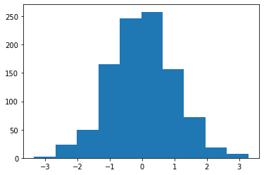
Plotting a histogram
- We can use the
hist()function inmatplotlibto plot a histogram
# Generate some random data
data = np.random.randn(1000)

ax = plt.hist(data)
plt.show()
Computing histograms as matrices
- The function
histogram()in thenumpymodule will count frequencies into bins and return the result as a 2-dimensional array.
np.histogram(data)
Defining new functions
def squared(x):
    return x ** 2

squared(5)
Local Variables
Variables created inside functions are local to that function.
They are not accessable to code outside of that function.
def squared(x):
    result = x ** 2
    return result

squared(5)
result
Functional Programming
Functions are first-class citizens in Python.
They can be passed around just like any other value.
squared
y = squared
y
y(5)
Mapping the elements of a collection
We can apply a function to each element of a collection using the built-in function
map().This will work with any collection: list, set, tuple or string.
This will take as an argument another function, and the list we want to apply it to.
It will return the results of applying the function, as a list.
list(map(squared, [1, 2, 3, 4]))
List Comprehensions
- Because this is such a common operation, Python has a special syntax to do the same thing, called a list comprehension.
[squared(i) for i in [1, 2, 3, 4]]
- If we want a set instead of a list we can use a set comprehension
{squared(i) for i in [1, 2, 3, 4]}
Cartesian product using list comprehensions
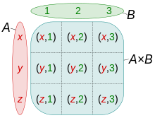 image courtesy of [Quartl](https://commons.wikimedia.org/wiki/User:Quartl)
The Cartesian product of two collections $X = A \times B$ can be expressed by using multiple for statements in a comprehension.
example
A = {'x', 'y', 'z'}
B = {1, 2, 3}
{(a,b) for a in A for b in B}
Cartesian products with other collections
- The syntax for Cartesian products can be used with any collection type.
first_names = ('Steve', 'John', 'Peter')
surnames = ('Smith', 'Doe')

[(first_name, surname) for first_name in first_names for surname in surnames]
Anonymous Function Literals
- We can also write anonymous functions.
- These are function literals, and do not necessarily have a name.
- They are called lambda expressions (after the $\lambda-$calculus).
list(map(lambda x: x ** 2, [1, 2, 3, 4]))
Filtering data
We can filter a list by applying a predicate to each element of the list.
A predicate is a function which takes a single argument, and returns a boolean value.
filter(p, X)is equivalent to $\{ x : p(x) \; \forall x \in X \}$ in set-builder notation.
list(filter(lambda x: x > 0, [-5, 2, 3, -10, 0, 1]))
We can use both filter() and map() on other collections such as strings or sets.
list(filter(lambda x: x > 0, {-5, 2, 3, -10, 0, 1}))
Filtering using a list comprehension
Again, because this is such a common operation, we can use simpler syntax to say the same thing.
We can express a filter using a list-comprehension by using the keyword
if:
data = [-5, 2, 3, -10, 0, 1]
[x for x in data if x > 0]
- We can also filter and then map in the same expression:
from numpy import sqrt
[sqrt(x) for x in data if x > 0]
The reduce function
- The
reduce()function recursively applies another function to pairs of values over the entire list, resulting in a single return value.
from functools import reduce
reduce(lambda x, y: x + y, [0, 1, 2, 3, 4, 5])
Big Data
The
map()andreduce()functions form the basis of the map-reduce programming model.Map-reduce is the basis of modern highly-distributed large-scale computing frameworks.
It is used in BigTable, Hadoop and Apache Spark.
See these examples in Python for Apache Spark.
Numerical Computing in Python
Overview
- Floating-point representation
- Arrays and Matrices with
numpy - Basic plotting with
matplotlib - Pseudo-random variates with
numpy.random
Representing continuous values
Digital computers are inherently discrete.
Real numbers $x \in R$ cannot always be represented exactly in a digital computer.
They are stored in a format called floating-point.
IEEE Standard 754 specifies a universal format across different implementations.
- As always there are deviations from the standard.
There are two standard sizes of floating-point numbers: 32-bit and 64-bit.
64-bit numbers are called double precision, are sometimes called double values.
IEEE floating-point calculations are performed in hardware on modern computers.
How can we represent aribitrary real values using only 32 bits?
Fixed-point verses floating-point
One way we could discretise continuous values is to represent them as two integers $x$ and $y$.
The final value is obtained by e.g. $r = x + y \times 10^{-5}$.
So the number $500.4421$ would be represented as the tuple $x = 500$, $y = 44210$.
The exponent $5$ is fixed for all computations.
This number represents the precision with which we can represent real values.
It corresponds to the where we place we place the decimal point.
This scheme is called fixed precision.
It is useful in certain circumstances, but suffers from many problems, in particular it can only represent a very limited range of values.
In practice, we use variable precision, also known as floating point.
Scientific Notation
Humans also use a form of floating-point representation.
In Scientific notation, all numbers are written in the form $m \times 10^n$.
When represented in ASCII, we abbreviate this
<m>e<n>, for example6.72e+11= $6.72 \times 10^{11}$.The integer $m$ is called the significand or mantissa.
The integer $n$ is called the exponent.
The integer $10$ is the base.
Scientific Notation in Python
- Python uses Scientific notation when it displays floating-point numbers:
print(672000000000000000.0)
Note that internally, the value is not represented exactly like this.
Scientific notation is a convention for writing or rendering numbers, not representing them digitally.
Floating-point representation
Floating point numbers use a base of $2$ instead of $10$.
Additionally, the mantissa are exponent are stored in binary.
Therefore we represent floating-point numbers as $m \times 2 ^ e$.
The integers $m$ (mantissa) and $e$ (exponent) are stored in binary.
The mantissa uses two's complement to represent positive and negative numbers.
- One bit is reserved as the sign-bit: 1 for negative, 0 for positive values.
The mantissa is normalised, so we assume that it starts with the digit $1$ (which is not stored).
Bias
We also need to represent signed exponents.
The exponent does not use two's complement.
Instead a bias value is subtracted from the stored exponent ($s$) to obtain the final value ($e$).
Double-precision values use a bias of $b = 1023$, and single-precision uses a bias value of $b = 127$.
The actual exponent is given by $e = s - b$ where $s$ is the stored exponent.
The stored exponent values $s=0$ and $s=1024$ are reserved for special values- discussed later.
The stored exponent $s$ is represented in binary without using a sign bit.
Double and single precision formats
The number of bits allocated to represent each integer component of a float is given below:
| Format | Sign | Exponent | Mantissa | Total |
|---|---|---|---|---|
| single | 1 | 8 | 23 | 32 |
| double | 1 | 11 | 52 | 64 |
By default, Python uses 64-bit precision.
We can specify alternative precision by using the numpy numeric data types.
Loss of precision
We cannot represent every value in floating-point.
Consider single-precision (32-bit).
Let's try to represent $4,039,944,879$.
Loss of precision
- As a binary integer we write $4,039,944,879$ as:
11110000 11001100 10101010 10101111
This already takes up 32-bits.
The mantissa only allows us to store 24-bit integers.
So we have to round. We store it as:
+1.1110000 11001100 10101011e+31
- Which gives us
+11110000 11001100 10101011 0000000
$= 4,039,944,960$
Ranges of floating-point values
In single precision arithmetic, we cannot represent the following values:
Negative numbers less than $-(2-2^{-23}) \times 2^{127}$
Negative numbers greater than $-2^{-149}$
Positive numbers less than $2^{-149}$
Positive numbers greater than $(2-2^{-23}) \times 2^{127}$
Attempting to represent these numbers results in overflow or underflow.
Effective floating-point range
| Format | Binary | Decimal |
|---|---|---|
| single | $\pm (2-2^{-23}) \times 2^{127}$ | $\approx \pm 10^{38.53}$ |
| double | $\pm (2-2^{-52}) \times 2^{1023}$ | $\approx \pm 10^{308.25}$ |
import sys
sys.float_info.max
sys.float_info.min
sys.float_info
Range versus precision
- With a fixed number of bits, we have to choose between:
- maximising the range of values (minimum to maximum) we can represent,
- maximising the precision with-which we can represent each indivdual value.
These are conflicting objectives:
- we can increase range, but only by losing precision,
- we can increase precision, but only by decreasing range.
Floating-point addresses this dilemma by allowing the precision to vary ("float") according to the magnitude of the number we are trying to represent.
Floating-point density
Floating-point numbers are unevenly-spaced over the line of real-numbers.
The precision decreases as we increase the magnitude.

Representing Zero
Zero cannot be represented straightforwardly because we assume that all mantissa values start with the digit 1.
Zero is stored as a special-case, by setting mantissa and exponent both to zero.
The sign-bit can either be set or unset, so there are distinct positive and negative representations of zero.
Zero in Python
x = +0.0
x
y = -0.0
y
- However, these are considered equal:
x == y
Infinity
Positive overflow results in a special value of infinity (in Python
inf).This is stored with an exponent consiting of all 1s, and a mantissa of all 0s.
The sign-bit allows us to differentiate between negative and positive overflow: $-\infty$ and $+\infty$.
This allows us to carry on calculating past an overflow event.
Infinity in Python
x = 1e300 * 1e100
x
x = x + 1
x
Negative infinity in Python
x > 0
y = -x
y
y < x
Not A Number (NaN)
Some mathematical operations on real numbers do not map onto real numbers.
These results are represented using the special value to
NaNwhich represents "not a (real) number".NaNis represented by an exponent of all 1s, and a non-zero mantissa.
NaN in Python
from numpy import sqrt, inf, isnan, nan
x = sqrt(-1)
x
y = inf - inf
y
Comparing nan values in Python
- Beware of comparing
nanvalues
x == y
- To test whether a value is
nanuse theisnanfunction:
isnan(x)
NaN is not the same as None
Nonerepresents a missing value.NaNrepresents an invalid floating-point value.These are fundamentally different entities:
nan is None
isnan(None)
Beware finite precision
x = 0.1 + 0.2
x == 0.3
x
Relative and absolute error
Consider a floating point number $x_{fp}$ which represents a real number $x \in \mathbf{R}$.
In general, we cannot precisely represent the real number; that is $x_{fp} \neq x$.
The absolute error $r$ is $r = x - x_{fp}$.
The relative error $R$ is:
Numerical Methods
In e.g. simulation models or quantiative analysis we typically repeatedly update numerical values inside long loops.
Programs such as these implement numerical algorithms.
It is very easy to introduce bugs into code like this.
Numerical stability
The round-off error associated with a result can be compounded in a loop.
If the error increases as we go round the loop, we say the algorithm is numerically unstable.
Mathematicians design numerically stable algorithms using numerical analysis.
Catastrophic Cancellation
Suppose we have two real values $x$, and $y = x + \epsilon$.
$\epsilon$ is very small and $x$ is very large.
$x$ has an exact floating point representation
However, because of lack of precision $x$ and $y$ have the same floating point representation.
- i.e. they are represented as the same sequence of 64-bits
Consider wheat happens when we compute $y - x$ in floating-point.
Catestrophic Cancellation and Relative Error
Catestrophic cancellation results in very large relative error.
If we calculate $y - x$ in floating-point we will obtain the result 0.
The correct value is $(x + \epsilon) - x = \epsilon$.
The relative error is
That is, the relative error is $100\%$.
This can result in catastrophy.
Catastrophic Cancellation in Python
x = 3.141592653589793
x
y = 6.022e23
x = (x + y) - y
x
Cancellation versus addition
- Addition, on the other hand, is not catestrophic.
z = x + y
z
The above result is still inaccurate with an absolute error $r \approx \pi$.
However, let's examine the relative error:
- Here we see that that the relative error from the addition is miniscule compared with the cancellation.
Floating-point arithemetic is nearly always inaccurate.
You can hardly-ever eliminate absolute rounding error when using floating-point.
The best we can do is to take steps to minimise error, and prevent it from increasing as your calculation progresses.
Cancellation can be catastrophic, because it can greatly increase the relative error in your calculation.
Use a well-tested library for numerical algorithms.
Avoid subtracting two nearly-equal numbers.
Especially in a loop!
Better-yet use a well-validated existing implementation in the form of a numerical library.
import numpy as np
- We can now use the functions defined in this package by prefixing them with
np.
Arrays
Arrays represent a collection of values.
In contrast to lists:
- arrays typically have a fixed length
- they can be resized, but this involves an expensive copying process.
- and all values in the array are of the same type.
- typically we store floating-point values.
- arrays typically have a fixed length
Like lists:
- arrays are mutable;
- we can change the elements of an existing array.
Arrays in numpy
Arrays are provided by the
numpymodule.The function
array()creates an array given a list.
import numpy as np
x = np.array([0, 1, 2, 3, 4])
x
Array indexing
- We can index an array just like a list
x[4]
x[4] = 2
x
Arrays are not lists
- Although this looks a bit like a list of numbers, it is a fundamentally different type of value:
type(x)
- For example, we cannot append to the array:
x.append(5)
Populating Arrays
- To populate an array with a range of values we use the
np.arange()function:
x = np.arange(0, 10)
print(x)
- We can also use floating point increments.
x = np.arange(0, 1, 0.1)
print(x)
Functions over arrays
- When we use arithmetic operators on arrays, we create a new array with the result of applying the operator to each element.
y = x * 2
y
- The same goes for numerical functions:
x = np.array([-1, 2, 3, -4])
y = abs(x)
y
Vectorized functions
Note that not every function automatically works with arrays.
Functions that have been written to work with arrays of numbers are called vectorized functions.
Most of the functions in
numpyare already vectorized.You can create a vectorized version of any other function using the higher-order function
numpy.vectorize().
vectorize example
def myfunc(x):
    if x >= 0.5:
        return x
    else:
        return 0.0

fv = np.vectorize(myfunc)
x = np.arange(0, 1, 0.1)
x
fv(x)
Testing for equality
Because of finite precision we need to take great care when comparing floating-point values.
The numpy function
allclose()can be used to test equality of floating-point numbers within a relative tolerance.It is a vectorized function so it will work with arrays as well as single floating-point values.
x = 0.1 + 0.2
y = 0.3
x == y
np.allclose(x, y)
Plotting with matplotlib
We will use a module called
matplotlibto plot some simple graphs.This module has a nested module called
pyplot.By convention we import this with the alias
plt.This module provides functions which are very similar to MATLAB plotting commands.
import matplotlib.pyplot as plt
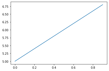
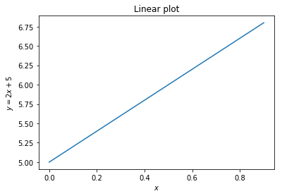
A simple linear plot
x = np.arange(0, 1, 0.1)
y = x*2 + 5
plt.plot(x, y)
plt.xlabel('$x$')
plt.ylabel('$y = 2x + 5$')
plt.title('Linear plot')
plt.show()
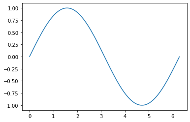
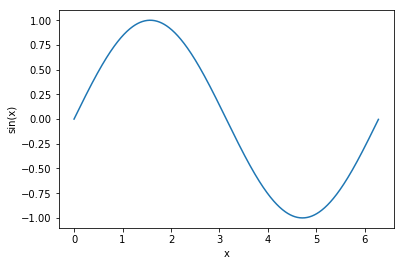
Plotting a sine curve
from numpy import pi, sin

x = np.arange(0, 2*pi, 0.01)
y = sin(x)
plt.plot(x, y)
plt.xlabel('x')
plt.ylabel('sin(x)')
plt.show()
Multi-dimensional data
Numpy arrays can hold multi-dimensional data.
To create a multi-dimensional array, we can pass a list of lists to the
array()function:
import numpy as np

x = np.array([[1,2], [3,4]])
x
Arrays containing arrays
A multi-dimensional array is an array of an arrays.
The outer array holds the rows.
Each row is itself an array:
x[0]
x[1]
- So the element in the second row, and first column is:
x[1][0]
Matrices
- We can create a matrix from a multi-dimensional array.
M = np.matrix(x)
M
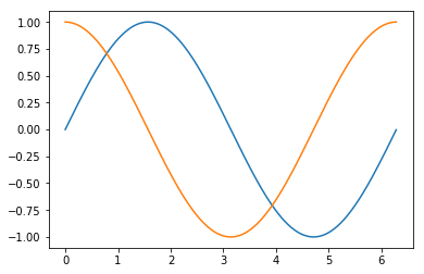
Plotting multi-dimensional with matrices
- If we supply a matrix to
plot()then it will plot the y-values taken from the columns of the matrix (notice the transpose in the example below).
from numpy import pi, sin, cos

x = np.arange(0, 2*pi, 0.01)
y = sin(x)
ax = plt.plot(x, np.matrix([sin(x), cos(x)]).T)
plt.show()
Performance
When we use
numpymatrices in Python the corresponding functions are linked with libraries written in C and FORTRAN.For example, see the BLAS (Basic Linear Algebra Subprograms) library.
These libraries are very fast.
Vectorised code can be more easily ported to frameworks like TensorFlow so that operations are performed in parallel using GPU hardware.
To compute the transpose $M^{T}$
M.T
To compute the inverse $M^{-1}$
M.I
Matrix Dimensions
- The total number of elements, and the dimensions of the array:
M.size
M.shape
len(M.shape)
Creating Matrices from strings
- We can also create arrays directly from strings, which saves some typing:
I2 = np.matrix('2 0; 0 2')
I2
- The semicolon starts a new row.
Matrix Multiplication
Now that we have two matrices, we can perform matrix multiplication:
M * I2
Matrix Indexing
- We can index and slice matrices using the same syntax as lists.
M[:,1]
Slices are references
- If we use this is an assignment, we create a reference to the sliced elements, not a copy.
V = M[:,1]  # This does not make a copy of the elements!
V
M[0,1] = -2
V
Copying matrices and vectors
- To copy a matrix, or a slice of its elements, use the function
np.copy():
M = np.matrix('1 2; 3 4')
V = np.copy(M[:,1])  # This does copy the elements.
V
M[0,1] = -2
V
Sums
One way we could sum a vector or matrix is to use a for loop.
vector = np.arange(0.0, 100.0, 10.0)
vector
result = 0.0
for x in vector:
    result = result + x
result
- This is not the most efficient way to compute a sum.
Efficient sums
Instead of using a
forloop, we can use a numpy functionsum().This function is written in the C language, and is very fast.
vector = np.array([0, 1, 2, 3, 4])
print(np.sum(vector))
Summing rows and columns
- When dealing with multi-dimensional data, the 'sum()' function has a named-argument
axiswhich allows us to specify whether to sum along, each rows or columns.
matrix = np.matrix('1 2 3; 4 5 6; 7 8 9')
print(matrix)
To sum along rows:
np.sum(matrix, axis=0)
To sum along columns:
np.sum(matrix, axis=1)
Cumulative sums
- Suppose we want to compute $y_n = \sum_{i=1}^{n} x_i$ where $\vec{x}$ is a vector.
import numpy as np
x = np.array([0, 1, 2, 3, 4])
y = np.cumsum(x)
print(y)
Cumulative sums along rows and columns
x = np.matrix('1 2 3; 4 5 6; 7 8 9')
print(x)
y = np.cumsum(x)
np.cumsum(x, axis=0)
np.cumsum(x, axis=1)
Cumulative products
- Similarly we can compute $y_n = \Pi_{i=1}^{n} x_i$ using
cumprod():
import numpy as np
x = np.array([1, 2, 3, 4, 5])
np.cumprod(x)
- We can compute cummulative products along rows and columns using the
axisparameter, just as with thecumsum()example.
Generating (pseudo) random numbers
- The nested module
numpy.randomcontains functions for generating random numbers from different probability distributions.
from numpy.random import normal, uniform, exponential, randint
Suppose that we have a random variable $\epsilon \sim N(0, 1)$.
In Python we can draw from this distribution like so:
epsilon = normal()
epsilon
- If we execute another call to the function, we will make a new draw from the distribution:
epsilon = normal()
epsilon
Pseudo-random numbers
Strictly speaking, these are not random numbers.
They rely on an initial state value called the seed.
If we know the seed, then we can predict with total accuracy the rest of the sequence, given any "random" number.
Nevertheless, statistically they behave like independently and identically-distributed values.
- Statistical tests for correlation and auto-correlation give insignificant results.
For this reason they called pseudo-random numbers.
The algorithms for generating them are called Pseudo-Random Number Generators (PRNGs).
Some applications, such as cryptography, require genuinely unpredictable sequences.
- never use a standard PRNG for these applications!
Managing seed values
In some applications we need to reliably reproduce the same sequence of pseudo-random numbers that were used.
We can specify the seed value at the beginning of execution to achieve this.
Use the function
seed()in thenumpy.randommodule.
Setting the seed
from numpy.random import seed

seed(5)
normal()
normal()
seed(5)
normal()
normal()
Drawing multiple variates
- To generate more than number, we can specify the
sizeparameter:
normal(size=10)
- If you are generating very many variates, this will be much faster than using a for loop
- We can also specify more than one dimension:
normal(size=(5,5))
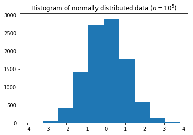
Histograms
- We can plot a histograms of randomly-distributed data using the
hist()function from matplotlib:
import matplotlib.pyplot as plt

data = normal(size=10000)
ax = plt.hist(data)
plt.title('Histogram of normally distributed data ($n=10^5$)')
plt.show()
Computing histograms as matrices
- The function
histogram()in thenumpymodule will count frequencies into bins and return the result as a 2-dimensional array.
import numpy as np
np.histogram(data)
np.mean(data)
np.var(data)
- These functions also have an
axisparameter to compute mean and variances of columns or rows of a multi-dimensional data-set.
Descriptive statistics with nan values
- If the data contains
nanvalues, then the descriptive statistics will also benan.
from numpy import nan
import numpy as np
data = np.array([1, 2, 3, 4, nan])
np.mean(data)
- To omit
nanvalues from the calculation, use the functionsnanmean()andnanvar():
np.nanmean(data)
Discrete random numbers
The
randint()function innumpy.randomcan be used to draw from a uniform discrete probability distribution.It takes two parameters: the low value (inclusive), and the high value (exclusive).
So to simulate one roll of a die, we would use the following Python code.
die_roll = randint(0, 6) + 1
die_roll
Just as with the
normal()function, we can generate an entire sequence of values.To simulate a Bernoulli process with $n=20$ trials:
bernoulli_trials = randint(0, 2, size = 20)
bernoulli_trials
Financial data with data frames
Data frames
The
pandasmodule provides a powerful data-structure called a data frame.It is similar, but not identical to:
- a table in a relational database,
- an Excel spreadsheet,
- a dataframe in R.
Loading data
Data frames can be read and written to/from:
- financial web sites
- database queries
- database tables
- CSV files
- json files
Beware that data frames are memory resident;
- If you read a large amount of data your PC might crash
- With big data, typically you would read a subset or summary of the data via e.g. a select statement.
Importing pandas
- The pandas module is usually imported with the alias
pd.
import pandas as pd
Series
A Series contains a one-dimensional array of data, and an associated sequence of labels called the index.
The index can contain numeric, string, or date/time values.
When the index is a time value, the series is a time series.
The index must be the same length as the data.
If no index is supplied it is automatically generated as
range(len(data)).
Creating a series from an array
import numpy as np
data = np.random.randn(5)
data
my_series = pd.Series(data, index=['a', 'b', 'c', 'd', 'e'])
my_series
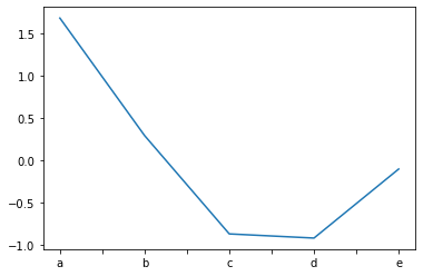
Plotting a series
We can plot a series by invoking the
plot()method on an instance of aSeriesobject.The x-axis will autimatically be labelled with the series index.
import matplotlib.pyplot as plt
my_series.plot()
plt.show()
Creating a series with automatic index
- In the following example the index is creating automatically:
pd.Series(data)
Creating a Series from a dict
d = {'a' : 0., 'b' : 1., 'c' : 2.}
my_series = pd.Series(d)
my_series
Indexing a series with []
Series can be accessed using the same syntax as arrays and dicts.
We use the labels in the index to access each element.
my_series['b']
- We can also use the label like an attribute:
my_series.b
Slicing a series
- We can specify a range of labels to obtain a slice:
my_series[['b', 'c']]
Arithmetic and vectorised functions
numpyvectorization works for series objects too.
d = {'a' : 0., 'b' : 1., 'c' : 2.}
squared_values = pd.Series(d) ** 2
squared_values
x = pd.Series({'a' : 0., 'b' : 1., 'c' : 2.})
y = pd.Series({'a' : 3., 'b' : 4., 'c' : 5.})
x + y
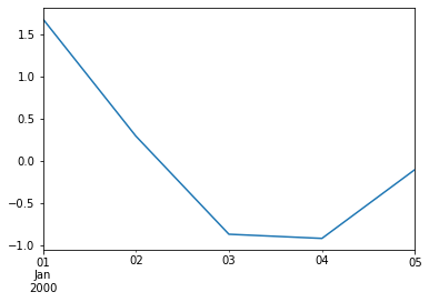
Time series
dates = pd.date_range('1/1/2000', periods=5)
dates
time_series = pd.Series(data, index=dates)
time_series
Plotting a time-series
ax = time_series.plot()
Missing values
Pandas uses
nanto represent missing data.So
nanis used to represent missing, invalid or unknown data values.It is important to note that this only convention only applies within pandas.
- Other frameworks have very different semantics for these values.
DataFrame
A data frame has multiple columns, each of which can hold a different type of value.
Like a series, it has an index which provides a label for each and every row.
Data frames can be constructed from:
- dict of arrays,
- dict of lists,
- dict of dict
- dict of Series
- 2-dimensional array
- a single Series
- another DataFrame
Creating a dict of series
series_dict = {
        'x' :
            pd.Series([1., 2., 3.], index=['a', 'b', 'c']),
        'y' :
            pd.Series([4., 5., 6., 7.], index=['a', 'b', 'c', 'd']),
        'z' :
            pd.Series([0.1, 0.2, 0.3, 0.4], index=['a', 'b', 'c', 'd'])
}

series_dict
Converting the dict to a data frame
df = pd.DataFrame(series_dict)
df
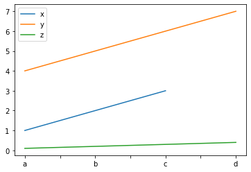
Plotting data frames
When plotting a data frame, each column is plotted as its own series on the same graph.
The column names are used to label each series.
The row names (index) is used to label the x-axis.
ax = df.plot()
Indexing
The outer dimension is the column index.
When we retrieve a single column, the result is a Series
df['x']
df['x']['b']
df.x.b
Projections
- Data frames can be sliced just like series.
- When we slice columns we call this a projection, because it is analogous to specifying a subset of attributes in a relational query, e.g.
SELECT x FROM table. - If we project a single column the result is a series:
slice = df['x'][['b', 'c']]
slice
type(slice)
Projecting multiple columns
- When we include multiple columns in the projection the result is a DataFrame.
slice = df[['x', 'y']]
slice
type(slice)
Vectorization
- Vectorized functions and operators work just as with series objects:
df['x'] + df['y']
df ** 2
Logical indexing
- We can use logical indexing to retrieve a subset of the data.
df['x'] >= 2
df[df['x'] >= 2]
Combining predicates
| operator | meaning |
|---|---|
& |
and |
| |
or |
~ |
not |
df[(df['x'] >= 2) & (df['y'] > 5)]
df[~((df['x'] >= 2) & (df['y'] > 5))]
Descriptive statistics
- To quickly obtain descriptive statistics on numerical values use the
describemethod.
df.describe()
Accessing a single statistic
- The result is itself a DataFrame, so we can index a particular statistic like so:
df.describe()['x']['mean']
Accessing the row and column labels
- The row labels (index) and column labels can be accessed:
df.index
df.columns
Head and tail
- Data frames have
head()andtail()methods which behave analgously to the Unix commands of the same name.
Financial data
Pandas was originally developed to analyse financial data.
We can download tabulated data in a portable format called Comma Separated Values (CSV).
import pandas as pd
googl = pd.read_csv('data/GOOGL.csv')
Examining the first few rows
When working with large data sets it is useful to view just the first/last few rows in the dataset.
We can use the
head()method to retrieve the first rows:
googl.head()
Examining the last few rows
googl.tail()
Parsing time stamps
- So far, the
Dateattribute is of type string.
googl.Date[0]
type(googl.Date[0])
Converting to datetime values
In order to work with time-series data, we need to construct an index containing time values.
Time values are of type
datetimeorTimestamp.We can use the function
to_datetime()to convert strings to time values.
pd.to_datetime(googl['Date']).head()
Setting the index
- Now we need to set the index of the data-frame so that it contains the sequence of dates.
googl.set_index(pd.to_datetime(googl['Date']), inplace=True)
googl.index[0]
type(googl.index[0])
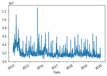
Plotting series
We can plot a series in a dataframe by invoking its
plot()method.Here we plot a time-series of the daily traded volume:
ax = googl['Volume'].plot()
plt.show()
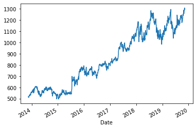
Adjusted closing prices as a time series
googl['Adj Close'].plot()
plt.show()
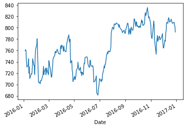
Slicing series using date/time stamps
We can slice a time series by specifying a range of dates or times.
Date and time stamps are specified strings representing dates in the required format.
googl['Adj Close']['1-1-2016':'1-1-2017'].plot()
plt.show()
Resampling
We can resample to obtain e.g. weekly or monthly prices.
In the example below the
'W'denotes weekly.See the documentation for other frequencies.
We group data into weeks, and then take the last value in each week.
For details of other ways to resample the data, see the documentation.
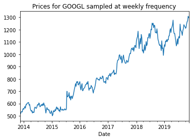
Resampled time-series plot
weekly_prices = googl['Adj Close'].resample('W').last()
weekly_prices.head()
weekly_prices.plot()
plt.title('Prices for GOOGL sampled at weekly frequency')
plt.show()
Converting prices to log returns
Log prices
log_prices = np.log(weekly_prices)
log_prices.head()
Differences
diffs = log_prices.diff()
diffs.head()
Remove missing values
weekly_rets = diffs.dropna()
weekly_rets.head()
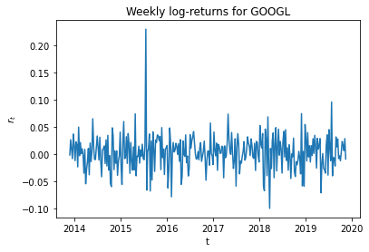
Log return time series plot
plt.plot(weekly_rets)
plt.xlabel('t'); plt.ylabel('$r_t$')
plt.title('Weekly log-returns for GOOGL')
plt.show()
Plotting a return histogram
weekly_rets.hist()
plt.show()
Descriptive statistics of returns
weekly_rets.describe()
Statistics and optimization with SciPy
The SciPy library
SciPy is a library that provides several modules for scientific computing.
You can read more about it by reading the reference guide.
It provides modules for:
- Solving optimization problems.
- Linear algebra.
- Interpolation.
- Statistical inference.
- Fourier transform.
- Numerical differentation and integration.
Overview
- loading data with pandas,
- computing returns,
- Quantile-Quantile (q-q) plots,
- The Jarque-Bera test for normally-distributed data,
- ordinary-least squares (OLS) regression.
- Portfolio optimization
Loading data
We will first obtain some data from Yahoo finance using the pandas library.
First we will import the functions and modules we need.
import matplotlib.pyplot as plt
import datetime
import pandas as pd
import numpy as np
Importing a CSV file
- Here we obtain price data on Microsoft Corporation Common Stock, so we specify the symbol MSFT.
def prices_from_csv(fname):
    df = pd.read_csv(fname)
    df.set_index(pd.to_datetime(df['Date']), inplace=True)
    return df
msft = prices_from_csv('data/MSFT.csv')
msft.head()
Data preparation
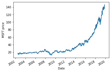
Daily prices
msft['Adj Close'].plot()
plt.ylabel('MSFT price')
plt.show()
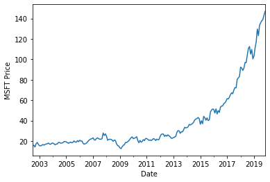
Converting to monthly data
We will resample the data at a frequency of one calendar month.
The code below takes the last price in every month.
daily_prices = msft['Adj Close']
monthly_prices = daily_prices.resample('M').last()
monthly_prices.plot()
plt.ylabel('MSFT Price')
plt.show()
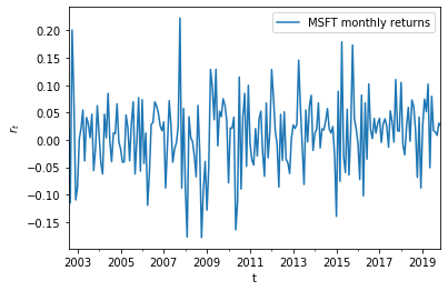
Calculating log returns
stock_returns = pd.DataFrame({'MSFT monthly returns': np.log(monthly_prices).diff().dropna()})
stock_returns.plot()
plt.xlabel('t'); plt.ylabel('$r_t$')
plt.show()
Exploratory data analysis
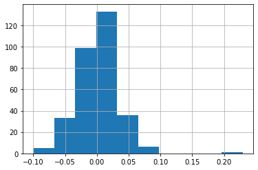
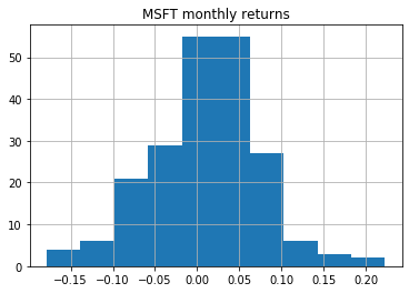
Return histogram
stock_returns.hist()
plt.show()
Descriptive statistics of the return distribution
stock_returns.describe()
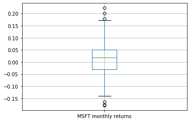
Summarising the distribution using a boxplot
stock_returns.boxplot()
plt.show()
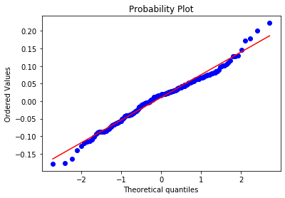
Q-Q plots
Quantile-Quantile (Q-Q) plots are a useful way to compare distributions.
We plot empirical quantiles against the quantiles computed the inverted c.d.f. of a specified theoretical distribution.
import numpy as np
import matplotlib.pyplot as plt
import scipy.stats as stats

stats.probplot(stock_returns.values[:,0], dist="norm", plot=plt)
plt.show()
Statistical Hypothesis Testing
The Jarque-Bera Test
The Jarque-Bera (JB) test is a statistical test that can be used to test whether a given sample was drawn from a normal distribution.
The null hypothesis is that the data have the same skewness (0) and kurtosis (3) as a normal distribution.
The test statistic is:
where $S$ is the sample skewness, $K$ is the sample kurtosis, and $n$ is the number of observations.
- It is implemented in
scipy.stats.jarque_bera().
References
Jarque, C. and Bera, A. (1980) “Efficient tests for normality, homoscedasticity and serial independence of regression residuals”, 6 Econometric Letters 255-259.
The Jarque-Bera test using a bootstrap
We can test against the null hypothesis of S=0 and K=3.
A finite sample can exhibit non-zero skewness and excess kurtosis simply due to sample noise, even if the distribution is Guassian.
What is the distribution of the sum of the squared sample skewness and kurtosis under repeated sampling?
We can answer this question using a Monte-Caro method called bootstrapping.
- Note that this is very expensive, and we would not always do this in practice (see the subsequent slides).
Bootstrap code
from scipy.stats import skew, kurtosis

def jb(n, s, k):
    return  n / 6. * (s**2 + (((k - 3.)**2) / 4.))

def jb_from_samples(n, bootstrap_samples):
    s = skew(bootstrap_samples)
    k = kurtosis(bootstrap_samples, fisher=False)
    return jb(n, s, k)
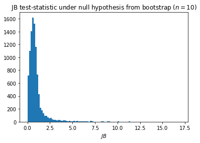
The distribution of the test-statistic under the null hypothesis
bootstrap_replications = 10000
n = 10  # Sample size
test_statistic_null = jb_from_samples(n, np.random.normal(size=(n, bootstrap_replications)))
plt.hist(test_statistic_null, bins=100)
plt.title('JB test-statistic under null hypothesis from bootstrap ($n=10$)'); plt.xlabel('$JB$')
plt.show()
The critical value
The 95-percentile can be computed from the bootstrap data.
This is called the critical value for $p= 0.05$.
critical_value = np.percentile(test_statistic_null, 95)
critical_value
This is the value of $JB_{crit}$ such that area underneath the p.d.f. over the interval $[0, JB_{crit}]$ sums to $0.95$ (95\% of the area under the curve).
The corresponding p-value is $1 - 0.95 = 0.05$.
Rejecting the null hypothesis
When we test an empirical sample, we compute its sample skewness and kurtosis, and the corresponding value of the test statistic $JB_{data}$.
We reject the null hypothesis iff. $JB_{data} > JB_{crit}$:
def jb_critical_value(n, bootstrap_samples, p):
    return np.percentile(jb_from_samples(n, bootstrap_samples), (1. - p) * 100.)

def jb_test(data_sample, bootstrap_replications=100000, p=0.05):
    sample_size = len(data_sample)
    bootstrap_samples = np.random.normal(size=(sample_size, bootstrap_replications))
    critical_value = jb_critical_value(sample_size, bootstrap_samples, p)
    empirical_jb = jb(sample_size, skew(data_sample), kurtosis(data_sample, fisher=False))
    return (empirical_jb > critical_value, empirical_jb, critical_value)
Test data from a normal distribution
x = np.random.normal(size=2000)
jb_test(x)
Test data from a log-normal distribution
jb_test(np.exp(x))
Critical-values from a Chi-Squared table
The code on the previous slide is not very efficient, since we have to perform a lengthly bootstrap operation each time we test a data sample.
For $n > 2000$, the distribution of the test statistic follows a Chi-squared distribution with two degrees of freedom ($k=2$), so we can look up the critical values for any given confidence level ($p$-value) using a Chi-Squared table.
For smaller $n$ we must resort to a bootstrap.
Producing a table of table critical values from a bootstrap
n = 10
bootstrap_samples = np.random.normal(size=(n, 300000))
confidence_levels = np.array([0.025, 0.05, 0.10, 0.20])
critical_values = np.vectorize(lambda p: jb_critical_value(n, bootstrap_samples, p))(confidence_levels)
critical_values_df = pd.DataFrame({'critical value (n=10)': critical_values}, index=confidence_levels)
critical_values_df.index.name = 'p-value'
critical_values_df
If we save this data-frame permanently, then we do not need to re-compute the critical value for the given sample size.
We can simply calculate the test-statistic from the data sample, and see whether the value thus obtained exceeds the critical value for the chosen level of confidence (p-value).
Using the jarque_bera function in scipy
The function
scipy.stats.jarque_bera()contains code already written to implement the Jarque-Bera (JB) test.It computes the p-value from the cdf. of the Chi-Squared distribution and the empirical test-statistic.
This assumes a large sample $n \geq 2000$.
The variable
test_statisticreturned below is the value of $JB$ calculated from the empirical data sample.If the p-value in the result is $\leq 0.05$ then we reject the null hypothesis at 95\% confidence.
The null hypothesis is that the data are drawn from a distribution with skew 0 and kurtosis 3.
import scipy.stats
x = np.random.normal(size=2000)
(test_statistic, p_value) = scipy.stats.jarque_bera(x)
print("JB test statistic = %f" % test_statistic)
print("p-value = %f" % p_value)
Testing the empirical data
len(stock_returns)
stats.jarque_bera(stock_returns)
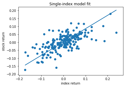
Estimating the single-index model
$$r_{i,t} - r_f = \alpha_i + \beta_i ( r_{m,t} - r_f) + \epsilon_{i,t}$$$$\epsilon_{i, t} \sim N(0, \sigma_i)$$- $r_{i,t}$ is return to stock $i$ in period $t$.
- $r_f$ is the risk-free rate.
- $r_{m,t}$ is the return to the market portfolio.
Elton, E. J., & Gruber, M. J. (1997). Modern portfolio theory, 1950 to date. Journal of Banking and Finance, 21(11–12), 1743–1759. https://doi.org/10.1016/S0378-4266(97)00048-4
nasdaq_index = prices_from_csv('data/^NDX.csv')
nasdaq_index.head()
Converting to monthly data
- As before, we can resample to obtain monthly data.
nasdaq_monthly_prices = nasdaq_index['Adj Close'].resample('M').last()
nasdaq_monthly_prices.head()
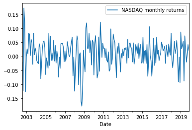
Plotting monthly returns
index_log_returns = pd.DataFrame({'NASDAQ monthly returns': np.log(nasdaq_monthly_prices).diff().dropna()})
index_log_returns.plot()
plt.show()
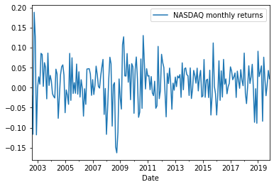
Converting to simple returns
index_simple_returns = np.exp(index_log_returns) - 1.
index_simple_returns.plot()
plt.show()
stock_simple_returns = np.exp(stock_returns) - 1.
Concatenating data into a single data frame
We will now concatenate the data into a single data fame.
We can use
pd.concat(), specifying an axis of 1 to merge data along columns.This is analogous to performing a
zip()operation.
comparison_df = pd.concat([index_simple_returns, stock_simple_returns], axis=1)
comparison_df.head()
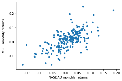
Scatter plots
We can produce a scatter plot to see whether there is any relationship between the stock returns, and the index returns.
There are two ways to do this:
- Use the function
scatter()inmatplotlib.pyplot - Invoke the
plot()method on a data frame, passingkind='scatter'
- Use the function
Scatter plots using the plot() method of a data frame
In the example below, the
xandynamed arguments refer to column numbers of the data frame.Notice that the
plot()method is able to infer the labels automatically.
comparison_df.plot(x=0, y=1, kind='scatter')
plt.show()
Computing the correlation matrix
- For random variables $X$ and $Y$, the Pearson correlation coefficient is:
Covariance and correlation of a data frame
- We can invoke the
cov()andcorr()methods on a data frame.
comparison_df.cov()
comparison_df.corr()
Comparing multiple attributes in a data frame
It is often useful to work with more than two variables.
We can add columns (attributes) to our data frame.
Many of the methods we are using will automatically incorporate the additional variables into the analysis.
Using a function to compute returns
- The code below defines a function defines a function which will return a data frame containing a single series of returns for the specified symbol, and sampled over the specified frequency.
def returns_df(symbol, frequency='M'):
df = prices_from_csv('data/%s.csv' % symbol)
prices = df['Adj Close'].resample(frequency).last()
column_name = symbol + ' returns (' + frequency + ')'
return pd.DataFrame({column_name: np.exp(np.log(prices).diff().dropna()) - 1.})
apple_returns = returns_df('AAPL')
apple_returns.head()
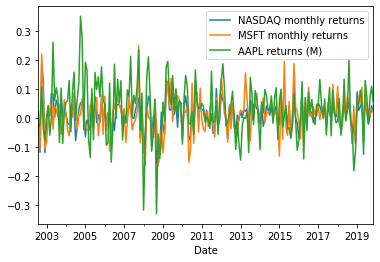
Adding another stock to the portfolio
comparison_df = pd.concat([comparison_df, apple_returns], axis=1)
comparison_df.head()
comparison_df.plot()
plt.show()
comparison_df.corr()
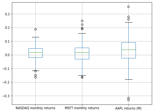
plt.figure(figsize=(8, 6))
comparison_df.boxplot()
plt.show()
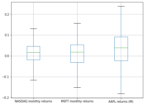
Boxplots without outliers
plt.figure(figsize=(8, 6))
comparison_df.boxplot(showfliers=False)
plt.show()
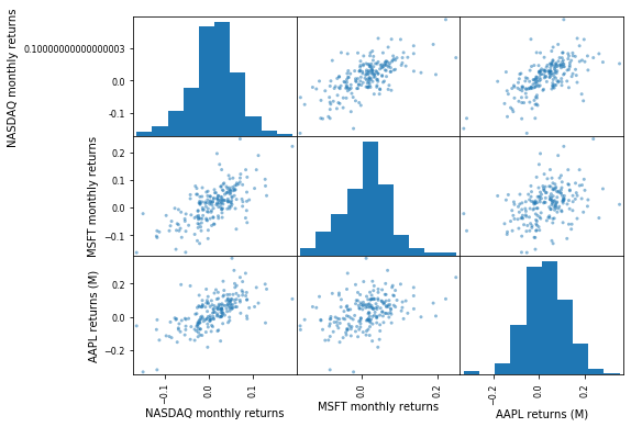
Scatter matrices
pd.plotting.scatter_matrix(comparison_df, figsize=(8, 6))
plt.show()
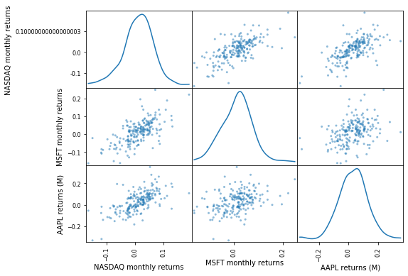
Scatter matrices with Kernel-density plots
- We can use Kernel density estimation (KDE) to plot an approximation of the pdf.
pd.plotting.scatter_matrix(comparison_df, diagonal='kde', figsize=(8, 6))
plt.show()
Ordinary-least squares
- For $n$ observations $(x_{1, j}, y_1), (x_{2, j}, y_2), \ldots, (x_{n, j}, y_n)$ over $j \in \{ 1, 2, \ldots p \}$ regressors:
Ordinary-least squares estimation in Python
- First we import the stats module:
import scipy.stats as stats
- Now we prepare the data set:
rr = 0.01 # risk-free rate
ydata = stock_simple_returns.values[:,0] - rr
xdata = index_simple_returns.values[:,0] - rr
regression_result = (beta, alpha, rvalue, pvalue, stderr) = \
stats.linregress(x=xdata, y=ydata)
print(regression_result)
Plotting the fitted model
plt.scatter(x=ydata, y=xdata)
plt.plot(ydata, alpha + beta * ydata)
plt.xlabel('index return')
plt.ylabel('stock return')
plt.title('Single-index model fit ')
plt.show()
Regressing attributes of a data frame
- First we will create a new data frame containing the excess returns.
excess_returns_df = comparison_df - rr
excess_returns_df.head()
Renaming the columns of a data frame
- We will now rename the columns to make the variable names easier to work with.
excess_returns_df.rename(columns={'NASDAQ monthly returns': 'index',
'MSFT monthly returns': 'msft',
'AAPL returns (M)': 'aapl'},
inplace=True)
excess_returns_df.head()
Fitting the model
import statsmodels.formula.api as sm
result = sm.ols(formula = 'msft ~ index', data=excess_returns_df).fit()
The full regression results
print(result.summary())
The intercept and coefficient
print(result.params)
coefficient = result.params['index']
coefficient
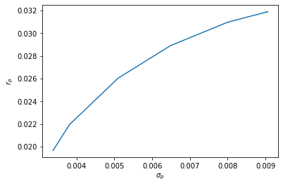
Portfolio optimization
- For a column vector $\mathbf{w}$ of portfolio weights, the portfolio return $r_p$ is given by:
- The portfolio variance $\sigma_p$ is given by:
where $\mathbf{K}$ is the covariance matrix.
Portfolio mean and variance in Python
- We can write the equation from the previous slide as a Python function:
def portfolio_mean_var(w, R, K):
portfolio_mean = np.mean(R, axis=0) * w
portfolio_var = w.T * K * w
return portfolio_mean.item(), portfolio_var.item()
- The
item()method is required to convert a one-dimensional matrix into a scalar.
Obtaining portfolio data in Pandas
portfolio = pd.concat([returns_df(s) for s in ['AAPL', 'ATVI', 'MSFT', 'VRSN', 'WDC']], axis=1)
portfolio.head()
Computing the covariance matrix
portfolio.cov()
Converting to matrices
R = np.matrix(portfolio)
K = np.matrix(portfolio.cov())
K
An example portfolio
- Let's construct a single portfolio by specifying a weight vector:
w = np.matrix('0.4; 0.2; 0.2; 0.1; 0.1')
w
np.sum(w)
portfolio_mean_var(w, R, K)
Optimizing portfolios
We can use the
scipy.optimizemodule to solve the portfolio optimization problem.First we import the module:
import scipy.optimize as sco
Defining an objective function
Next we define an objective function.
This function will be minimized.
def portfolio_performance(w_list, R, K, risk_aversion):
w = np.matrix(w_list).T
mean, var = portfolio_mean_var(w, R, K)
return risk_aversion * var - (1 - risk_aversion) * mean
Computing the performance of a given portfolio
def uniform_weights(n):
return [1. / float(n)] * n
uniform_weights(5)
portfolio_performance(uniform_weights(5), R, K, risk_aversion=0.5)
Finding optimal portfolio weights
def optimal_portfolio(R, K, risk_aversion):
n = R.shape[1]
constraints = ({'type': 'eq', 'fun': lambda x: np.sum(x) - 1})
bounds = tuple( (0,1) for asset in range(len(w)))
result = sco.minimize(portfolio_performance, uniform_weights(n), args=(R, K, risk_aversion),
method='SLSQP', bounds=bounds, constraints=constraints)
return np.matrix(result.x).T
optimal_portfolio(R, K, risk_aversion=0.5)
Computing the Pareto frontier
- First we define our risk aversion coefficients
risk_aversion_coefficients = np.arange(0.0, 1.0, 0.1)
risk_aversion_coefficients
The optimal portfolios
optimal_portfolios = [optimal_portfolio(R, K, ra) for ra in risk_aversion_coefficients]
optimal_portfolios[0]
optimal_portfolios[1]
The efficient frontier
pareto_frontier = np.matrix([portfolio_mean_var(w, R, K) for w in optimal_portfolios])
pareto_frontier
Plotting the Pareto frontier
plt.plot(pareto_frontier[:, 1], pareto_frontier[:, 0])
plt.xlabel('$\sigma_p$'); plt.ylabel('$r_p$')
plt.show()
Monte-Carlo Methods
Quantitative Models
A mathematical model uses variables to represent quantities in the real-world.
- e.g. security prices
Variables are related to each other through mathematical equations.
Variables can be divided into:
- Input variables: parameters (independent variables)
- Inititial conditions: parameters which specify the initial values of in a time-varying (dynamic) model.
- Output variables: dependent-variables (e.g. payoff of an option).
- Input variables: parameters (independent variables)
Monte-Carlo Methods
Financial models are typically stochastic.
Stochastic models make use of random variables.
If the dependent variables are stochastic, we typically want to compute their expectation.
- Note, however, that in some models, dependent variables are deterministic, even when parameters are random.
If the parameters are stochastic, we can use Monte-Carlo methods to estimate the expected values of dependent variables.
The Monte-Carlo Casino
"Monte-Carlo" was the secret code-name of a project which used the earliest Monte-Carlo methods to solve problems of neurton-diffusion during the development of the first-atomic bomb.
It was named after the Monte-Carlo casino.
Pseudo-code
We will illustrate a simple Monte-Carlo method for analysing a stochastic model.
We will make use of pseudo-code.
Pseudo-code is written for people.
It is not executable by machines.
It is written to illustrate exactly how something is done.
Exact specifications of the steps required to compute mathematical values are called algorithms.
Pseudo-code can be used to write down algorithms.
A simple Monte-Carlo method
Here we consider a simple model with one input variable $X$, and one output variable $Y$, related by a function $Y = f(X)$.
$X$ and $Y$ are random variables.
$X$ is iid. distributed with some known distribution.
We want to compute the expected value of the dependent variable $E(Y)$.
We do so by drawing a random sample of $n$ random variates $( x_1, x_2, \ldots, x_n )$ from the specified distribution.
We map these values onto a sample $\mathbf{y}$ of the dependent variable $Y$: $\mathbf{y} = ( f(x_1), f(x_2), \ldots, f(x_n) )$.
We can use the sample mean $\bar{\mathbf{y}} = \sum_i f(x_i) / n$ to estimate $E(Y)$.
Provided that $n$ is sufficiently large, our estimate will be accurate by the law of large numbers.
$\bar{\mathbf{y}}$ is called the Monte-Carlo estimator.
In Pseudo-code
- The pseudo-code below illustrates the method specified on the previous slide using iteration:
sample = []
for i in range(n):
x = draw_random_value(distribution)
y = f(input_variable)
sample.append(y)
result = mean(sample)
- We can write this more concisely using a comprehension:
inputs = draw_random_value(distribution, size=n)
result = mean([f(x) for x in inputs])
A Monte-Carlo algorithm for computing $\pi$
- Inscribe a circle in a square.
- Randomly generate points $(X, Y$) in the square.
- Determine the number of points in the square that are also in the circle.
- Let $R$ be the number of points in the circle divided by the number of points in the square, then $\pi = 4 \times E(R)$.
See this tutorial.
import numpy as np
def f(x, y):
if x*x + y*y < 1:
return 1.
else:
return 0.
n = 1000000
X = np.random.random(size=n)
Y = np.random.random(size=n)
pi_approx = 4 * np.mean([f(x, y) for (x, y) in zip(X,Y)])
print("Pi is approximately %f" % pi_approx)
Monte-Carlo Integration
The expectation of a random variable $X \in \mathbb{R}$ with pdf. $f(x)$ can be written:
$$ E[X] = \int_{-\infty}^{+\infty} x f(x) \; dx $$For a continuous uniform distribution over $U(0, 1)$, the pdf. is $f(x) = 1$, and:
$$ E[X] = \int_{0}^{1} x \; dx $$Estimating $\pi$ using Monte-Carlo integration
Consider:
$$E[\sqrt{1 - X^2}] = \int_0^1 \sqrt{1 - x^2} \; dx$$If we draw a finite random sample $x_1, x_2, \ldots, x_n$ from $U(0, 1)$, then
\begin{eqnarray} \bar{\mathbf{x}} \approx E[X] & = & \int_0^1 \sqrt{1 - x^2} dx \end{eqnarray}\begin{eqnarray} \int \sqrt{1 - x^2} dx & = & \frac{1}{2} ( x \sqrt{1-x^2} + \arcsin(x) ) .\\ \end{eqnarray}Therefore:
$$\bar{\mathbf{x}} \approx E[X] = \frac{\pi}{4}$$Estimation error
By the law of large numbers $\lim_{n \rightarrow \infty} \bar{\mathbf{x}} = E(X)$.
However, for finite values of $n$ we will have an estimation error.
Can we quantify the estimation error as a function of $n$?
Computing the error numerically
If we draw from a standard normal distribution, we know that $E(X) = 0$.
Therefore, we can easily compute the estimation error in any given sample.
The error for a small random sample.
Here $X \sim N(0, 1)$, and we draw a random sample $\mathbf{x} = (x_1, x_2, \ldots, x_n)$ of size $n=5$.
We will compute $\epsilon_\mathbf{x} = | \bar{\mathbf{x}} - E(X) | = | \bar{\mathbf{x}} |$
x = np.random.normal(size=5)
x
np.mean(x)
estimation_error = np.abs(np.mean(x))
estimation_error
Computing the error for different samples
- If we draw a different sample, will the error be different or the same?
Sample 1
x = np.random.normal(size=5)
estimation_error = np.abs(np.mean(x))
estimation_error
Sample 2
x = np.random.normal(size=5)
estimation_error = np.abs(np.mean(x))
estimation_error
Sample 3
x = np.random.normal(size=5)
estimation_error = np.abs(np.mean(x))
estimation_error
Errors are random variables
We can see that the error $\epsilon_{\mathbf{x}}$ is itself a random variable.
How can we compute $E(\epsilon_{\mathbf{x}})$?
Monte-Carlo estimation of the sampling error
def sampling_error(n):
errors = [np.abs(np.mean(np.random.normal(size=n))) \
for i in range(100000)]
return np.mean(errors)
sampling_error(5)
- Notice that this estimate is relatively stable:
sampling_error(5)
sampling_error(5)
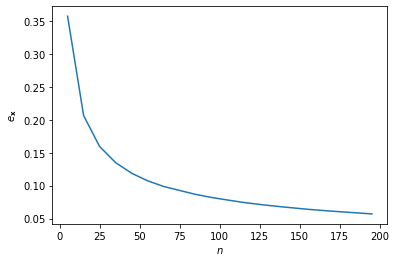
Monte-Caro estimation of the standard error
- We can now examine the relationship between sample size $n$ and the expected error using a Monte-Carlo method.
import matplotlib.pyplot as plt
n = np.arange(5, 200, 10)
plt.plot(n, np.vectorize(sampling_error)(n))
plt.xlabel('$n$'); plt.ylabel('$e_\mathbf{x}$')
plt.show()
The sampling distribution of the mean
The variance in the error occurs because the sample mean is a random variable.
What is the distribution of the sample mean?
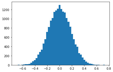
The sampling distribution of the mean
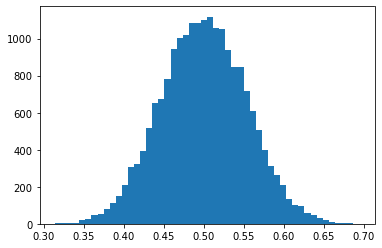
- Let's fix the sample size at $n=30$, and look at the empirical distribution of the sample means.
# Sample size
n = 30
# Number of repeated samples
N = 20000
means_30 = [np.mean(np.random.normal(size=n)) for i in range(N)]
ax = plt.hist(means_30, bins=50)
plt.show()
The sampling distribution of the mean for $n=30$
- Now let's do this again for a variable sampled from a different distribution: $X \sim U(0, 1)$.
# Sample size
n = 30
# Number of repeated samples
N = 20000
means_30_uniform = [np.mean(np.random.uniform(size=n)) for i in range(N)]
ax = plt.hist(means_30_uniform, bins=50)
plt.show()
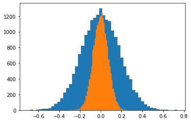
Increasing the sample size $n=200$
# Sample size
n = 200
means_200 = [np.mean(np.random.normal(size=n)) for i in range(N)]
ax1 = plt.hist(means_30, bins=50)
ax2 = plt.hist(means_200, bins=50)
plt.show()
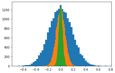
Increasing the sample size $n=1000$
# Sample size
n = 1000
means_1000 = [np.mean(np.random.normal(size=n)) for i in range(N)]
ax1 = plt.hist(means_30, bins=50)
ax2 = plt.hist(means_200, bins=50)
ax3 = plt.hist(means_1000, bins=50)
plt.show()
The sampling distribution of the mean
In general the sampling distribution of the mean approximates a normal distribution.
If $X \sim N(\mu, \sigma^2)$ then $\bar{\mathbf{x}_n} \sim N(\mu, \frac{\sigma^2}{n})$.
The standard error of the mean is $\sigma_{\bar{\mathbf{x}}} = \frac{\sigma}{\sqrt{n}}$.
Therefore sample size must be quadrupled to achieve half the measurement error.
Summary
Monte-Carlo methods can be used to analyse quantitative models.
Any problem in which the solution can be written as an expectation of random variable(s) can be solved using a Monte-Carlo approach.
We write down an estimator for the problem; a variable whose expectation represents the solution.
We then repeatedly sample input variables, and calculate the estimator numerically (in a computer program).
The sample mean of this variable can be used as an approximation of the solution; that is, it is an estimate.
The larger the sample size, the more accurate the estimate.
There is an inverse-square relationship between sample size and the estimation error.
Random walks in Python
A Simple Random Walk
Imagine a board-game in which we move a counter either up or down on an infinite grid based on the flip of a coin.
We start in the center of the grid at position $y_1 = 0$.
Each turn we flip a coin. If it is heads we move up one square, otherwise we move down.
How will the counter behave over time? Let's simulate this in Python.
First we create a variable $y$ to hold the current position
y = 0
Movements as Bernoulli trials
- Now we will generate a Bernoulli sequence representing the moves
- Each movement is an i.i.d. discrete random variable $\epsilon_t$ distributed with $p(\epsilon_t = 0) = \frac{1}{2}$ and $p(\epsilon_t = 1) = \frac{1}{2}$.
- We will generate a sequence $( \epsilon_1, \epsilon_2, \ldots, \epsilon_{t_{max}} )$ such movements, with $t_{max} = 100$.
- The time variable is also discrete, hence this is a discrete-time model.
- This means that time values can be represented as integers.
Simulating a Bernoulli process in Python
import numpy as np
from numpy.random import randint
max_t = 100
movements = randint(0, 2, size=max_t)
print(movements)
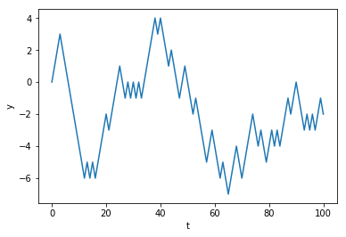
An integer random-walk in Python
- Each time we move the counter, we move it in the upwards direction if we flip a 1, and downwards for a 0.
- So we add 1 to $y_t$ for a 1, and subtract 1 for a $0$.
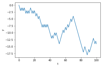
an integer random-walk using a loop
import numpy as np
import matplotlib.pyplot as plt
from numpy.random import randint, normal, uniform
max_t = 100
movements = randint(0, 2, size=max_t)
y = 0
values = [y]
for movement in movements:
if movement == 1:
y = y + 1
else:
y = y - 1
values.append(y)
plt.xlabel('t')
plt.ylabel('y')
ax = plt.plot(values)
plt.show()
A random-walk as a cumulative sum
- Notice that the value of $y_t$ is simply the cumulative sum of movements randomly chosen from $-1$ or $+1$.
- So if $p(\epsilon = -1) = \frac{1}{2}$ and $p(\epsilon = +1) = \frac{1}{2}$ then
- We can define our game as a simple stochastic process : $y_t = \sum_{t=1}^{t_{max}} \epsilon_t$
- We can use numpy's
where()function to replace all zeros with $-1$.
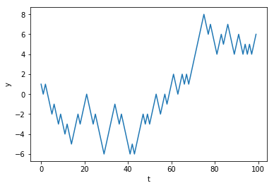
an integer random-walk using an accumulator
t_max = 100
random_numbers = randint(0, 2, size=t_max)
steps = np.where(random_numbers == 0, -1, +1)
y = 0
values = [0]
for step in steps:
y = y + step
values.append(y)
plt.xlabel('t')
plt.ylabel('y')
ax = plt.plot(values)
A random-walk using arrays
- We can make our code more efficient by using the
cumsum()function instead of a loop. - This way we can work entirely with arrays.
- Remember that vectorized code can be much faster than iterative code.
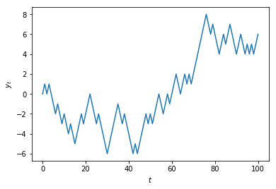
an integer random-walk using vectorization
# Vectorized random-walk with arrays to improve efficiency
t_max = 100
random_numbers = randint(0, 2, size=t_max)
steps = np.where(random_numbers == 0, -1, +1)
values = np.cumsum(steps)
plt.xlabel('t')
plt.ylabel('y')
ax = plt.plot(values)
Using concatenate to prepend the initial value
If we want to include the initial position $y_0 = 0$, we can concatenate this value to the computed values from the previous slide.
The
numpy.concatenate()function takes a single argument containing a sequence of arrays, and returns a new array which contains all values in a single array.
plt.plot(np.concatenate(([0], values)))
plt.xlabel('$t$')
plt.ylabel('$y_t$')
plt.show()
Multiple realisations of a stochastic process
Because we are making use of random numbers, each time we execute this code we will obtain a different result.
In the case of a random-walk, the result of the simulation is called a path.
Each path is called a realisation of the model.
We can generate multiple paths by using a 2-dimensional array (a matrix).
Suppose we want $n= 10$ paths.
In Python we can pass two values for the size argument in the
randint()function to specify the dimensions (rows and columns):
t_max = 100
n = 10
random_numbers = randint(0, 2, size=(t_max, n))
steps = np.where(random_numbers == 0, -1, +1)
Using cumsum()
We can then tell cumsum() to sum the rows using the axis argument:
values = np.cumsum(steps, axis=0)
values = np.concatenate((np.matrix(np.zeros(n)), values), axis=0)
plt.xlabel('$t$')
plt.ylabel('$y_t$')
ax = plt.plot(values)
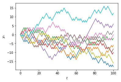
Multiplicative Random Walks
The series of values we have looked at do not closely resememble how security prices change over time.
In order to obtain a more realistic model of how prices change over time, we need to multiply instead of add.
Let $r_t$ denote an i.i.d. random variable distributed $r_t \sim N(0, \sigma^2)$
Define a strictly positive intitial value $y_0 \in \mathbf{R}$; e.g. $y_0 = 10$.
Subsequent values are given by $y_t = y_{t-1} \times (1 + r_t)$
We can write this as a cumulative product:
$y_t = y_0 \times \Pi_{t=1}^{t_{max}} \epsilon_t$
initial_value = 100.0
random_numbers = normal(size=t_max) * 0.005
multipliers = 1 + random_numbers
values = initial_value * np.cumprod(multipliers)
plt.xlabel('$t$')
plt.ylabel('$y_t$')
ax = plt.plot(np.concatenate(([initial_value], values)))
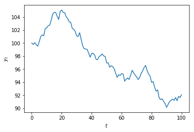
Random walk variates as a time-series
- Now let's plot the random perturbations over time
plt.xlabel('$t$')
plt.ylabel('$r_t$')
ax = plt.plot(random_numbers)
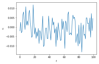
Gross returns
If we take $100 \times \epsilon_t$, then these represent the percentage changes in the value at discrete time intervals.
If the values represent prices that have been adjusted to incorporate dividends, then the multipliers are called simple returns.
The gross return is obtained by adding 1.
plt.xlabel('$t$')
plt.ylabel('$r_t$')
ax = plt.plot(random_numbers + 1)
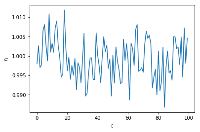
Continuously compounded, or log returns
- A simple return $R_t$ is defined as
$R_t = (y_t - y_{t-1}) / y_{t-1} = y_{t} / y_{t-1} - 1$
where $y_t$ is the adjusted price at time $t$.
The gross return is $R_t + 1$
A continuously compounded return $r_t$, or log-return, is defined as:
$r_t = \log(y_t / y_{t-1}) = \log(y_t) - \log(y_{t-1})$
- In Python:
from numpy import diff, log
prices = values
log_returns = diff(log(prices))
Aggregating returns
Simple returns aggregate across assets- the return on a portfolio of assets is the weighted average of the simple returns of its individual securities.
Log returns arregate across time.
If return in year one is $r_1 = \log(p_1 / p_0) = \log(p_1) - \log(p_0)$
- and return in year two is $r_2 = \log(p_2 / p_1) = \log(p_2) - \log(p_1)$,
- then return over two years is $r_1 + r_2 = \log(p_2) - \log(p_0)$
Converting between simple and log returns
- A simple return $R_t$ can be converted into a log-return $r_t$:
$r_t = \log(R_t + 1)$
Comparing simple and log returns
For small values of $r_t$ then $R_t \approx r_t$.
We can examine the error for larger values:
simple_returns = np.arange(-0.75, +0.75, 0.01)
log_returns = np.log(simple_returns + 1)
plt.xlim([-1.5, +1.5])
plt.ylim([-1.5, +1.5])
plt.plot(simple_returns, log_returns)
x = np.arange(-1.5, 1.6, 0.1)
plt.xlabel('R')
plt.ylabel('r')
ax = plt.plot(x, x)
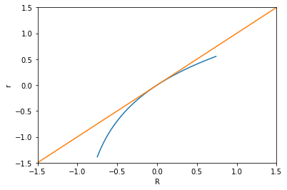
A discrete multiplicative random walk with log returns
Let $r_t$ denote a random i.i.d. variable distributed $r_t \sim N(0, \sigma^2)$
Then $y_t = y_0 \times \operatorname{exp}(\sum_{t=1}^{t_{max}} r_t)$
Plotting a single realization
from numpy import log, exp, cumsum
t_max = 100
volatility = 1e-2
initial_value = 100.
r = normal(size=t_max) * np.sqrt(volatility)
y = initial_value * exp(cumsum(r))
plt.xlabel('$t$')
plt.ylabel('$y_t$')
ax = plt.plot(np.concatenate(([initial_value], y)))
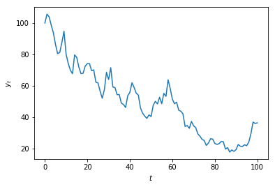
Multiple realisations of a multiplicative random-walk
- Let's generate $n=10$ realisations of this process:
def random_walk(initial_value = 100, n = 10,
t_max = 100, volatility = 0.005):
r = normal(size=(t_max+1, n)) * np.sqrt(volatility)
return np.concatenate((np.matrix([initial_value] * n),
initial_value * exp(np.cumsum(r, axis=0))))
plt.xlabel('$t$')
plt.ylabel('$y_t$')
ax = plt.plot(random_walk(n=10))
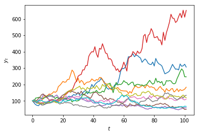
Geometric Brownian Motion
- For a continuous-time process, we use Geometric Brownian Motion (GBM):
- As a cumulative sum:
GBM with multiple paths in Python
def gbm(sigma, r, k, t_max, S0, I=1):
z = np.random.normal(size=(k-1, I))
dt = t_max/k
y = sigma * np.sqrt(dt)*z + (r - sigma**2 / 2.) * dt
return S0 * np.exp(np.cumsum(y, axis=0))
Plotting multiple realizations of GBM
sigma = 0.05; r = 0.01; k = 100; t_max = 10.; S0 = 100.
T = np.arange(0, t_max - t_max/k, t_max/k)
ax = plt.plot(T, gbm(sigma, r, k, t_max, S0, I=50))
plt.xlabel('$t$'); plt.ylabel('$S_t$'); plt.show()
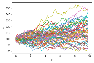
Monte-Carlo simulation for option pricing
Options
An option gives the right to buy (call) or sell (put) an underlying stock at a prespecified price, called the strike price, at a specified date, or period.
- A European option specifies a single date.
- An American option specifies a period.
Options can also specify an index, in which case they are settled in cash.
People selling options are called option writers.
People buying options are the option holders.
Payoff to an option holder
The payoff to an option holder depends on the index price $S_t$ when the option is exercised.
For a European option with strike price $K$, and maturity date $T$:
- If the index is below the strike, the option is worthless.
- Otherwise the holder receives the difference between the index price and the strike price: $S_T - K$.
Therefore the payoff to the option is:
Outcomes
- In-the-money (ITM):
- a call (put) is in-the-money if $ S > K (S < K) $.
- At-the-money (ATM):
- an option is at-the-money if $S \approx K$.
- Out-of-the-money (OTM):
- a call (put) is out-of-the-money if $ S < K (S > K) $.
import numpy as np
import matplotlib as mpl
import matplotlib.pyplot as plt
K = 8000 # Strike price
S = np.arange(7000, 9000, 100) # index level values
h = np.maximum(S - K, 0) # inner values of call option
Plotting the payoff function
plt.plot(S, h, lw=2.5) # plot inner values at maturity
plt.xlabel('index level $S_t$ at maturity'); plt.ylabel('inner value of European call option')
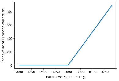
Parameters which affect the inner-value
Initial price level of the index $S_0$.
Volatility of the index $\sigma$.
The return(s) of the index.
Time-to-maturity $T$.
Risk-neutral assumptions
When all of the following assumptions hold:
- no arbitrage,
- complete markets (no transaction costs and perfect information),
- law of one price (assets with identical risk and return have a unique price)
Risk-neutral parameters
we can price options without having to take account of investors' risk-preferences using only the following parameters:
- Initial price level of the index $S_0$.
- Volatility of the index $\sigma$.
- Time-to-maturity $T$.
- The risk-free rate $r$.
Monte-Carlo option valuation
For a European option, the inner-value is not path-dependent.
Under risk-neutral pricing, we use Geometric Brownian Motion (GBM) with:
- where $r$ is the risk-free rate.
Non-path dependent algorithm to estimate the inner-value:
- Draw $I$ random numbers $z_1, z_2, \ldots, z_I$ from the standard normal distribution.
For $i \in \{1, 2, \ldots, I\}$:
i). Calculate index level at maturity by simulating geometric Brownian motion using the above equation.
ii). Compute the inner-value of the option $h_T = \max(S_T - K, 0)$.
iii). Discount back to the present at the risk-free rate $r$, giving the present value: $$C_i = e^{-rT} h_T.$$
Output the final estimate by computing the Monte-Carlo estimator $\bar{\mathbf{C}} = \frac{\sum_{i=1}^I C_i}{I}$
Monte-Carlo valuation of European call option in Python
In the following we use the following parameterization of the model: initial index price $S_0 = 100$, strike price $K=105$, time-to-maturity $T=1$, risk-free rate $r=0.02$, index volatility $\sigma=0.02$, number of independent realizations $I=10^5$.
from numpy import sqrt, exp, cumsum, sum, maximum, mean
from numpy.random import standard_normal
# Parameters
S0 = 100.; K = 105.; T = 1.0
r = 0.02; sigma = 0.1; I = 100000
# Simulate I outcomes
S = S0 * exp((r - 0.5 * sigma ** 2) * T + sigma * sqrt(T) *
standard_normal(I))
# Calculate the Monte Carlo estimator
C0 = exp(-r * T) * mean(maximum(S - K, 0))
print("Estimated present value is %f" % C0)
Asian (average-value) option
The payoff of an asian option is determined by the average of the price of the underlying over a pre-defined period of time.
Payoff for a fixed-strike Asian call option:
where:
$$ A(0, T) = \frac{1}{T} \int_0^T S_t dt $$If we let $t_i = i \times \frac{T}{n} \; i \in {0, 1, 2, \ldots, n}$:
$$ A(0, T) \approx \frac{1}{n} \sum_{i=0}^{n-1} S_{t_i} $$- The payoff is path dependent, and therefore we need to simulate intermediate values of $S_t$.
Path-dependent Monte-Carlo option pricing
- To simulate GBM at $M$ evenly spaced time intervals $t_i$ with $\Delta_T = T/M$:
Algorithm for path-dependent option pricing
- Draw $I \times M$ random numbers from the standard normal distribution.
For $i \in \{1, 2, \ldots, I\}$:
i). Calculate index level at times $t_i \in \{\Delta_T, 2\Delta_T, \ldots, T\}$ by simulating geometric Brownian motion with drift $\mu = r$ and volatility $\sigma$ using the equation for $S_{t_k}$.
ii). Estimate the inner-value of the option $\hat{h}_T = \frac{1}{T} \sum_{i=1}^M S_{t_i}$.
iii). Discount back to the present at the risk-free rate $r$, giving the present value: $$C_i = e^{-rT} \hat{h}_T.$$
Output the final estimate by computing the Monte-Carlo estimator $\bar{\mathbf{C}} = \frac{\sum_{i=1}^I C_i}{I}$
Monte-Carlo valuation of Asian fixed-strike call option in Python
In the following we use the following parameterization of the model: initial index price $S_0 = 100$, time-to-maturity $T=1$, number of time-steps $M=200$, risk-free rate $r=0.02$, index volatility $\sigma=0.1$, number of independent realizations $I=10^5$.
from numpy import sqrt, exp, cumsum, sum, maximum, mean
from numpy.random import standard_normal
# Parameters
S0 = 100.; T = 1.0; r = 0.02; sigma = 0.1
M = 200; dt = T / M; I = 100000
def inner_value(S):
""" Inner value for a fixed-strike Asian call option """
return mean(S, axis=0)
# Simulate I paths with M time steps
S = S0 * exp(cumsum((r - 0.5 * sigma ** 2) * dt + sigma * sqrt(dt) *
standard_normal((M + 1, I)), axis=0))
# Calculate the Monte Carlo estimator
C0 = exp(-r * T) * mean(inner_value(S))
print("Estimated present value is %f" % C0)
Estimating Value-At-Risk (VaR) in Python
Value-at-Risk (VaR)
Value at risk (VaR) is a methodology for computing a risk measurement on a portfolio of investments.
It is defined over:
- a duration of time, e.g. one day.
- a confidence level (or equivalent percentage) $\alpha$.
The $VaR_{\alpha}$ over duration $T$ is the maximum possible loss during $T$, excluding outcomes whose probability is less than $\alpha$, according to our model.
Value-at-Risk (VaR)
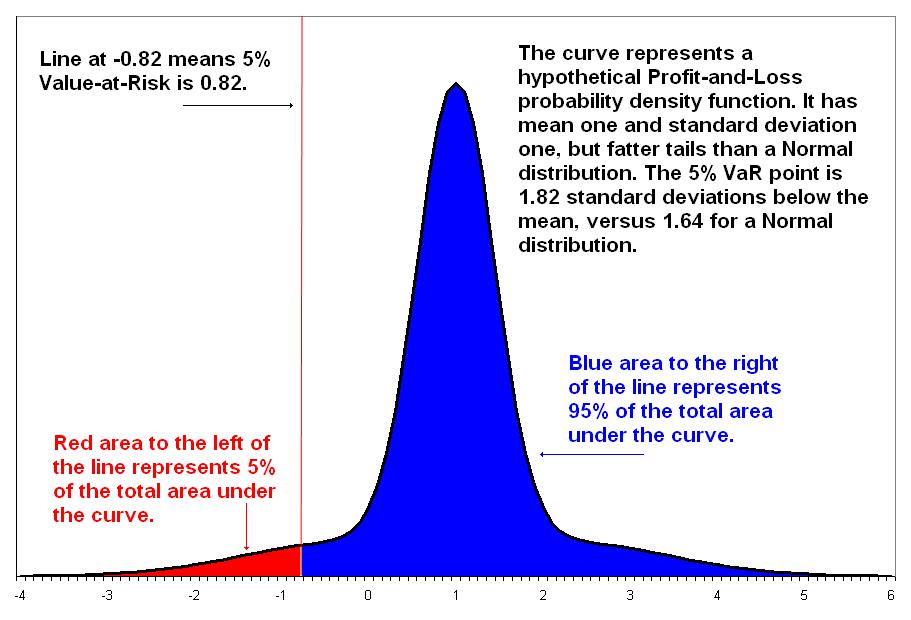
Mathematical definition
- Value at Risk with confidence $\alpha$ can be defined
where $X$ is a random variable representing the value of the portfolio, with cumulative distribution function $F_X$.
The $VaR_{\alpha}(X)$ is simply the negative of the $\alpha$-quantile.
We typically assume mark-to-market accounting, and so the value of the portfolio is determined from fair market prices.
Quantiles, Quartiles and Percentiles
0 quartile = 0 quantile = 0 percentile
1 quartile = 0.25 quantile = 25 percentile
2 quartile = .5 quantile = 50 percentile (median)
3 quartile = .75 quantile = 75 percentile
4 quartile = 1 quantile = 100 percentile
Computing quantiles in Python
- First we will generate some random data.
import numpy as np
# Draw values sampled iid from standard normal distribution
data = np.random.normal(size=100000)
import matplotlib.pyplot as plt
ax = plt.hist(data, bins=100)
plt.show()
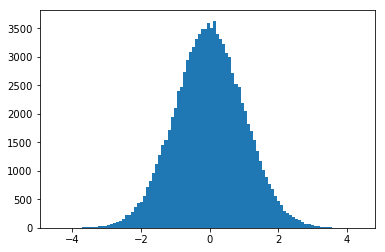
Computing quantiles in Python
# Compute the 5th-percentile
np.percentile(data, q=5)
Computing several percentiles
for p in range(1, 6):
print("The %d-percentile is %f" % (p, np.percentile(data, q=p)))
Estimating VaR
The VaR depends on the distribution of a random variable, e.g. the price of an index, over a specified period of time.
How can we estimate the quantiles of this distribution?
Estimating VaR
Common methods:
Variance/Covariance method.
Historical simulation- bootstrap from historical data.
Monte-Carlo simulation.
Historical simulation
To calculate $VaR_{\alpha}(X)$ with sampling interval $\Delta_t$ over $T = n \times \Delta_t$ using a total of $N$ bootstrap samples:
Assuming that the returns are stationary over the entire period, obtain a large sample of historical prices for the components of the portfolio or index.
Convert the prices into returns with frequency $1/\Delta_t$.
For every $i \in \{1, \ldots, N\}$:
Randomly choose $n$ returns $r_1, r_2, \ldots, r_n$ with replacement.
Compute $P_i | (r_1, r_2, \ldots, r_n)$ - the profit and loss of the investment given these returns.
Compute $Q(\alpha)$ from the sample $\mathbf{P}$, where $Q$ is the quantile function.
Random choices in Python
We can use the function
choice()from thenumpymodule to choose randomly from a set of values.To choose a single random value:
import numpy as np
data = np.random.randint(1, 6+1, size=20)
data
np.random.choice(data, replace=True)
np.random.choice(data, replace=True)
Generating a sequence of choices
- We can think of this as a simple bootstrap model of a dice:
np.random.choice(data, size=5, replace=True)
Bootstrapping from empirical data
Typically we will collect real-world (empirical) data from a random process whose true distribution is unknown.
In Finance, we can bootstrap from historical returns.
Obtaining returns for the Nikkei 225 index
import datetime
from pandas_datareader import data
start = datetime.datetime(2015, 1, 1)
end = datetime.datetime(2016, 1, 1)
n225 = data.DataReader("^N225", "yahoo", start, end)
returns = np.diff(np.log(n225["Adj Close"]))
plt.plot(returns)
plt.xlabel('t')
plt.ylabel('r')
plt.show()
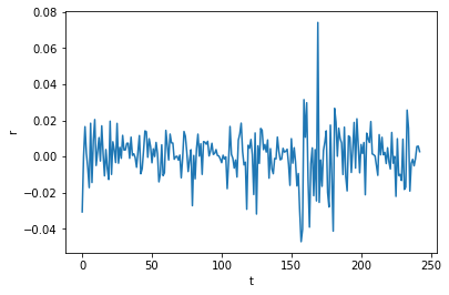
Simulating returns
- We will now simulate the returns over the next five days:
num_days = 5
simulated_returns = \
np.random.choice(returns, size=num_days, replace=True)
simulated_returns
Simulating prices
initial_price = 100.
prices = initial_price * np.exp(np.cumsum(simulated_returns))
plt.plot(prices)
plt.xlabel('t')
plt.ylabel('price')
plt.show()
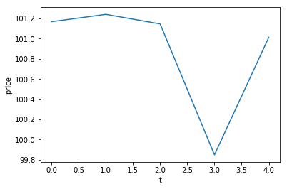
Multiple realisations
- If we perform this simulation again, will we obtain the same result?
First simulation
num_days = 5
simulated_returns = \
np.random.choice(returns, size=num_days, replace=False)
prices = initial_price * np.exp(np.cumsum(simulated_returns))
plt.plot(prices)
plt.xlabel('t')
plt.ylabel('price')
plt.show()
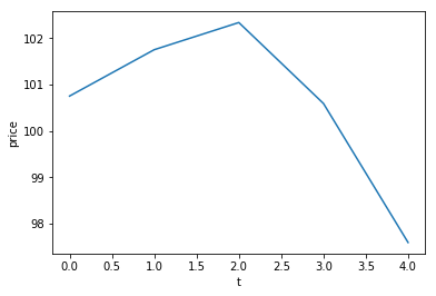
Second simulation
num_days = 5
simulated_returns = \
np.random.choice(returns, size=num_days, replace=False)
prices = initial_price * np.exp(np.cumsum(simulated_returns))
plt.plot(prices)
plt.xlabel('t')
plt.ylabel('price')
plt.show()
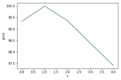
Third simulation
num_days = 5
simulated_returns = \
np.random.choice(returns, size=num_days, replace=False)
prices = initial_price * np.exp(np.cumsum(simulated_returns))
plt.plot(prices)
plt.xlabel('t')
_ = plt.ylabel('price')
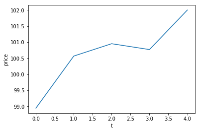
Many realisations - the distribution of the final price
def final_price():
num_days = 20
simulated_returns = \
np.random.choice(returns, size=num_days, replace=True)
prices = initial_price * np.exp(np.cumsum(simulated_returns))
return prices[-1]
num_samples = 100000
prices = [final_price() for i in range(num_samples)]
plt.hist(prices, bins=100)
plt.show()
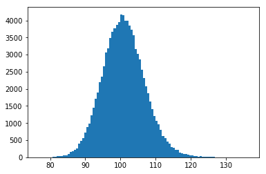
The distribution of the profit and loss
def profit_and_loss(final_price):
return 1200000. * (final_price - initial_price)
p_and_l = np.vectorize(profit_and_loss)(prices)
plt.hist(p_and_l, bins=100)
plt.show()
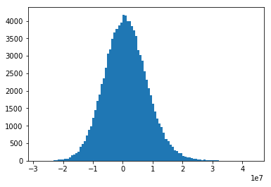
The quantiles of the profit and loss
for p in range(1, 6):
print("The %.2f-quantile is %.4f" % (p/100., np.percentile(p_and_l, q=p)))
What is the 5% Value-At-Risk?
import locale
var = -1 * np.percentile(p_and_l, q=5)
print("5%%-VaR is %.4f" % var)